Shortcut to seniority
Home
Go to main page
Section level: Junior
A journey into the programming realm
Section level: Intermediate
The point of no return
Section level: Senior
Leaping into the unknown

Go to main page
A journey into the programming realm
The point of no return
Leaping into the unknown
An algorithm is a set of instructions to execute in a specific given order. Any work to be done can be thought as a series of steps.
A greedy algorithm has only one shot to compute the optimal solution, so one characteristic is that it never goes back to reverses the decision.
A greedy algorithm is always making the choice that seems to be the best at that moment.
In other words, this means that a locally-optimal choice is made, which will hopefully lead to a globally-optional solution to our problem.
Creation of a greedy algorithm:
Problem: You have a T time to do the work, and you are required to do the maximum number of jobs.
So, how would you make the maximum number of jobs in a given time? By doing only the smallest task possible, for as much as possible.
Input:
Data to use:
Operations to perform:
Repeat this as long as current time is smaller or equal to T (final time).
Let's take an example.
Input:
Preparation: Sort the array.
| Iteration | Value picked | Current time | Jobs done |
|---|---|---|---|
| 1st | - | 0 | 0 |
| 2nd | 1 | 0 + 1 = 1 | 1 |
| 3rd | 2 | 1 + 2 = 3 | 2 |
| 4th | 3 | 3 + 3 = 6 | 3 |
After the 4th iteration, current time (6) is bigger than our max time T (4). Thus, the maximum number of jobs that can be performed in such time is 3.
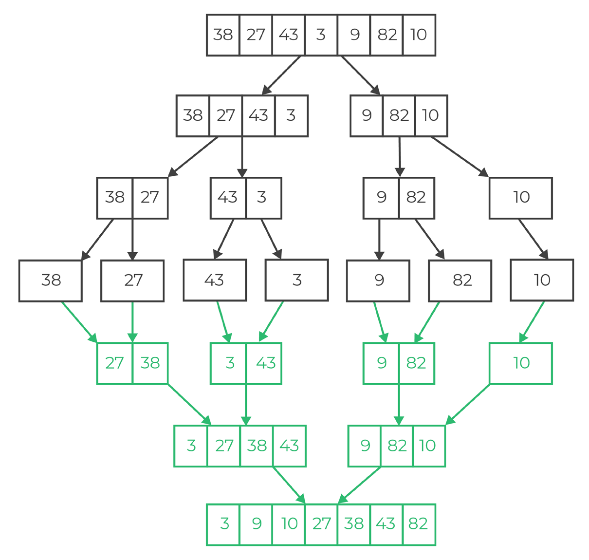
A typical divide and conquer algorithm solves a problem through three steps:

Dynamic programming is a technique that is based on a recurrent formula and one or multiple states. A sub-solution of the problem is constructed from previously found ones. (express the value of a function in terms of other values of that function).
The trick behind Dynamic Programming is that we trade space for time (instead of calculating all the states takes a lot of time but no space, and we take up space for results of sub-problems to save time).
Most Dynamic programming problems can be categorized into two types:
Optimization problems expect you to find a solution so that the value of a function is minimized or maximized. Combination problems expect you to figure out the number of ways to do something, or the probability of an event to happen.
Dynamic Programming problems should be resolved through the following schema:
In Top-down, you start building the solution right away by explaining how you build it from smaller solution. In Bottom-up, you start with the small solutions, and then build up.
Analogy:
Bottom up – I’m going to learn programming. Afterwards, I will start practicing. Afterwards, I will participate in contests. Afterwards, I’ll practice further and try to improve. Afterwards, I’ll be a great coder.
Top Down – I’l be a great coder. How? I’ll practice further and try to improve. How? I’ll participate in contests. How? I’ll start practicing. How? I’m going to learn programming.
Memoization is an optimization technique used to speed up applications by storing the results of an expensive function call and returning the cached result when the same input occurs again.
Whenever we need a solution to a subproblem, we look into the lookup table. If it’s there, we retrieve it, and otherwise, we calculate the value and add the result in the lookup table to be easily retrieved later on.
                                                        int fibonacci_topDown(int n, vector<int>& lookup_table) {
                                                        if (n == 0) return 0;
                                                        if (n == 1) return 1;
                                                        if (lookup_table[n] != 0) {
                                                            return lookup_table[n];
                                                        }
                                                        else {
                                                            lookup_table[n] = fibonacci_topDown(n - 1, lookup_table) +
                                                                                fibonacci_topDown(n - 2, lookup_table);

                                                            return lookup_table[n];
                                                        }
                                                        }

                                                        int main() {
                                                        int value = 10;
                                                        vector<int> lookup_table(value + 1, 0);

                                                        cout << fibonacci_topDown(value, lookup_table);
                                                        return 0;
                                                        }
In our case, the lookup table is found on line 17. We need to make sure we allocate enough memory to store the results.
First, we check the value of n in the lookup table (Lines 4-5). If the value is not found in the lookup table, we calculate it based on the previous results (Lines 8-9).
In the bottom-up approach, we calculate the small values, and then build larger values from them.
                                                        int fibonacci_bottomUp(int x) {
                                                        vector<int> results_table;
                                                        results_table.push_back(0);
                                                        results_table.push_back(1);

                                                        for (int i = 2; i <= x; i++) {
                                                            results_table.push_back(results_table[i - 1] + results_table[i - 2]);
                                                        }
                                                        return results_table[x];
                                                        }
Line 2 contains the results table, in which we add the values for 0 and 1 (Lines 3-4).
For each value starting from 2 to x, we add in the results table the solution from previously calculated values (Line 7).
Backtracking is a technique for solving problems recursively. It builds the solution by providing candidates, and it removes the candidate when it fails to satisfy the problem constraints. This usually results in visiting a previous stage of the process, and exploring new possibilities from that step.
Backtracking is used to solve three types of problems:
Let’s give an example.
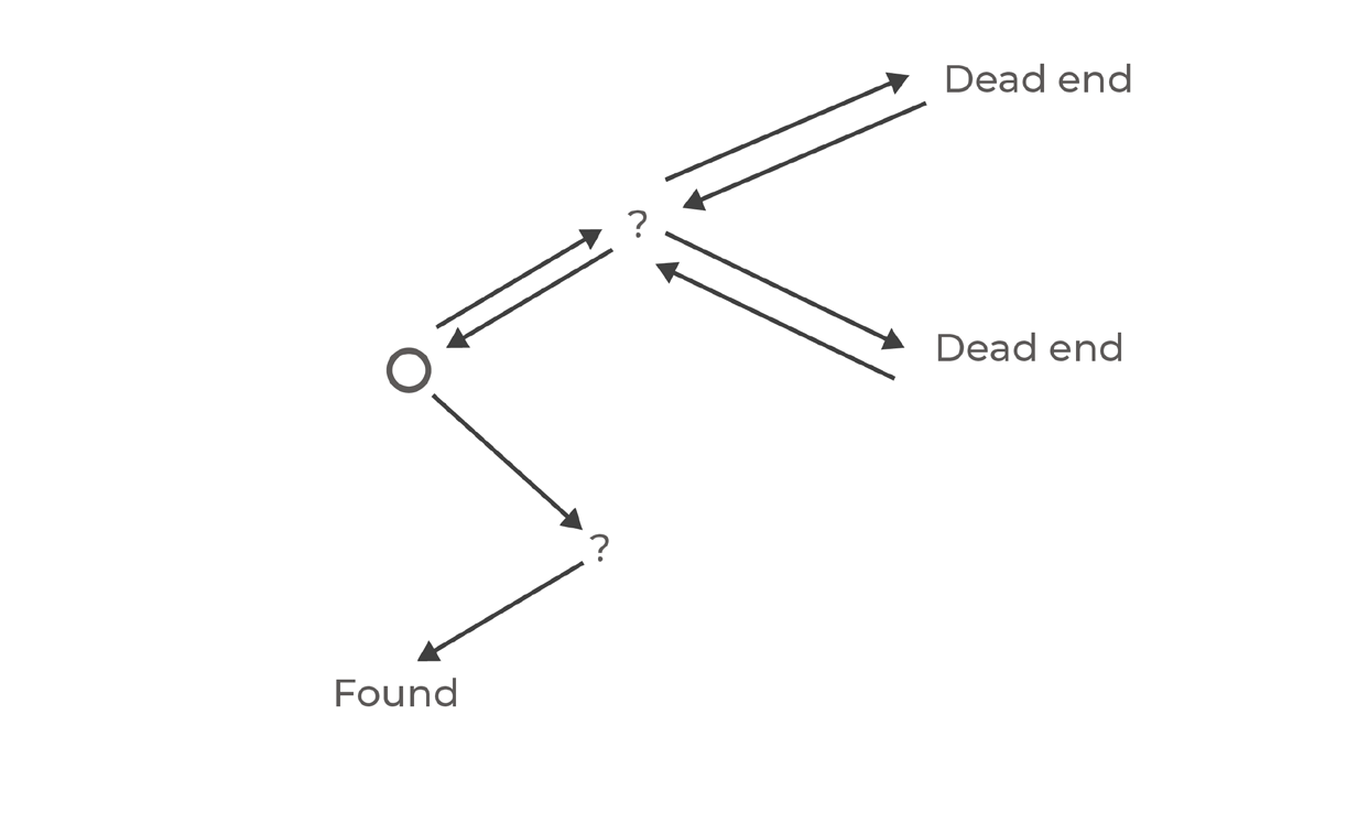
Assuming we are in a maze and we need to find our way out – we start moving in our path. In case there’s a bifurcation – we need to make a choice where we should go.
With backtracking + recursion, we simply choose to go everywhere.
We set left as our current road, and we move on that road. If we encounter a dead-end, we move back to the bifurcation, we set right as our current road, and we move on to that road. Each decision creates more sub-problems, and in most of them, we backtrack and revert our decision.

In code, this usually requires setting a value, calling the same function again, and in case the function returns fail, we unset the value and continue with the next option. The pseudo-code for backtracking (general algorithm) is at follows:
                                            Prerequisites: Data input (items in a vector, for example)

                                            For each item from Input
                                            if (constraints are valid)
                                                select the item
                                                result = recursive call for the rest of the problem

                                            if (result)
                                                return true
                                            else
                                                deselect the item

                                            return false
What we’re really doing is that we take each item one by one, check if the constraints are valid if we take such item, and we call the function again with the new information taking in. If at some point, the constraints are invalid, we deselect the item and check for the next one. The function should have a finish condition at start, if we reached the step we wanted, and should return false if it exhausted all the items without any success.
The most important thing in backtracking is the selection of the item and deselection of it in case it doesn’t satisfy the problem constraints.
An example of platform is the operating system, so we can include windows-related code only if we’re building the binary for windows, for example.
A pointer references a location in memory.
CPU cache is a small storage space that keeps the most frequently used data in order to reduce the accesses to the main memory.
Except for languages that contain garbage collector (which automatically frees memory that is no longer referenced).
NULL refer to the absence of a value, which means that it is not the same as having the value 0.
A Complete binary tree is a binary tree in which all nodes except leaves have two children, and the last level has all keys as left as possible.