Shortcut to seniority

Big O notation

Big O notation helps us determine how complex an operation is. It provides information on how long an operation will take, based on the size of the data. It can also be used as a complexity measurement.

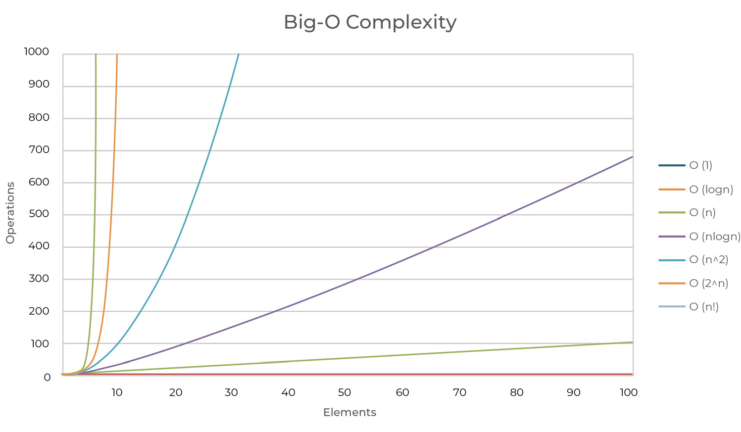
image with caption — Figure 23 - Algorithm concepts - Big O notation

The following table contain a list of the common O notations, from fastest (best) to slowest (worst).

Notation	Name	Example
O(1)	Constant	Operations occur at the `same speed`, independent of the data set. Example: null pointer check, comparing a given value to a constant
O(log n)	Logarithmic	Operations take `slightly longer`, as the size of the data set increases. Example: Finding an item in a sorted data set, using binary search
O(n)	Linear	Operations take longer and they are `directly proportioned` to the data set size Example: adding all the values within a container
O(n log n)	Linearithmic	As the data set doubles in size, operations take longer `by an increasing multiplier of one` Example: Quick sort
O(n²)	Quadratic	Each time data set doubles in size, the operations take four `times longer` Example: Two nested loops through the container (a for inside another for, from 1 to length of data)
O(2ⁿ)	Exponential	For every new element added in the data set, operations take `twice as long` Example: brute force
O(n!)	Quadratic	Operations take `n! times longer` directly proportioned to the size of the data Example: Calculating fibonacci numbers recursively

O comes from the Order of the function (growth rate), while n is the length of the data we work with.

Given the following formula:
f(n) = 8n⁵ – 3n⁴ + 6:
As n approaches infinity (for very large sets of data), 8n⁵ is the only one that actually matters, so all the lesser terms will simply drop. The constants drop as well, so the formula have a growth rate of O(n⁵).

Time complexity

The running time describes how many operations an algorithm must do before it completes.

For the next example, the growth rate is O(1), which means that the lookup is constant, no matter how big the container is.


                                                        vector<int> items = { 1, 2, 3, 4, 5, 6 };      
                                                            
                                                        bool isValueAtIndex(int index, int value) {      
                                                        return items[index] == value;      
                                                        }

For the next example, the growth rate is O(n) because, for a vector with n=1000 (1000 elements), the number of operations will also be 1000.


                                                        vector<int> items = { 1, 2, 3, 4, 5, 6 };      
                                                        int sum = 0;  
                                                        
                                                        int calculateSum() {      
                                                        for (int i = 0; i < items.size(); ++i) {  
                                                            sum += items[i];  
                                                        }  
                                                        return sum;  
                                                        }

For the next example, the growth rate is O(n²) because, for a vector with n=10 (10 elements), the number of operations will be 10².

For each number i from 0 to 9 (Line 4)
For each number j from 0 to 9 (Line 5)
Display the values on screen([0][0], [0][1], …[9][9])


                                                        vector<int> items = { 1, 2, 3, 4, 5, 6 };      
                                                            
                                                        void printItemsAsMatrix() {    
                                                        for (int i = 0; i < items.size(); ++i) {    
                                                            for (int j = 0; j < items.size(); ++j) {    
                                                            print(i, j);    
                                                            }    
                                                        }    
                                                        }    
                                                            
                                                        void print(int i, int j) {    
                                                        cout << "[" << i << "][" << j << "]";    
                                                        }

Space complexity

The space complexity describes how much space must be allocated to run the algorithm. For any algorithm, memory may be used for variables (constant, temporary variables), instruction, or execution.

Space Complexity is the sum of Auxiliary space and Input space. Auxiliary space is the extra/temporary space that is used by the algorithm during its execution, whereas the Input space refer to the data received as input.

To calculate the space complexity, we need to know the memory required for the type of variables, which generally is different for different operating systems.


                                            int function() {    
                                            int a = 10, b = 5, c = 5;    
                                            int sum = a + b + c;    
                                            
                                            return sum;    
                                            }

Let’s assume that the space requirement for an int is 4 bytes.

Variables a,b,c and sum are integers, so they will take 4 bytes each, and that number will not change based on input, so 16 is the total number of bytes required by the function.

Because the space requirements is fixed, we call it to be constant.


                                            vector<int> copy(const vector<int>& input) {  
                                            vector<int> output;  

                                            for(int i = 0; i < input.size(); i++) {       
                                                output.push_back(input[i]);     
                                            }    
                                            return output;    
                                            }

In the above example, we receive a vector and we copy each element of that vector into a new one.

Therefore, assuming the size of an integer is 4 bytes, we will need 4*n bytes of space for the elements, where n is the size of the original vector.

The memory is linearly increased based on the size of the vector, so the space complexity is linear => O(n).

Sorting

Sorting means rearranging the elements within a data structure, in an ordered sequence, based on a specific criteria.
Sorting is required in order to improve the efficiency of the search (lookup), merging, or processing data.
The opposite operation of sorting is called shuffling, and it implies rearranging a sequence of items in a random order.

There are two types of sorting algorithms: integer sorts, and comparison sorts.

Let’s provide a simple example.
Assuming we have the following information about a given set of items:

Fruit	Available units	Price / kg
Apple	1	2 $
Banana	15	1.4 $
Orange	3	5 $

Because sorting is done based on a specific criteria, we can choose how we want to display the items to the user.
For example, if we want to display in a descending order, based on the price, we would get the following table:

Fruit	Available units	Price / kg
Orange	3	5 $
Apple	1	2 $
Banana	15	1.4 $

Sorting is usually performed before an algorithm that has sorting as a prerequisite. If the items are already sorted, we don’t need to iterate through the entire data structure to find if a value is present in the data structure – if we check the middle of the structure directly and the value is smaller than what we’re searching for, because the items are sorted (meaning that all the lowest values will be at the start and all the highest values will be at the end), we know that the item we’re searching for is not in the first half.

This concept is called binary search, we’ll talk about it in the next chapter.

Recursion

Recursion refer to a function that is calling itself.

Recursion as concept is quite easy to grasp, but it’s difficult to write a recursive solution – at least not on the first try, and that is because it involves a different way of thinking.

A recursive solution is one where the solution to a problem is reached through recursion.

If we write a function that returns the sum of all numbers from 1 to 9, you could write it like this:


                                            int sum(int final) {    
                                                int sum = 0;    
                                                for (int i = 0; i < final; ++i)     
                                                    sum += i;    
                                                
                                                return sum;    
                                            }

With recursion, you would write it like this:


                                            int sum(int final, int current) {      
                                            if (current == final)       
                                                return current;      
                                                
                                            return current + sum(final, current + 1);      
                                            }      
                                                
                                            int total = sum(4, 0);

It works, but it’s ugly and hard to read. That’s because we needed to keep track of the current sum.
Let’s change the parameter and exit condition so it will start from the number and decrease to 0.


                                            int sum(int current) {    
                                            if (current == 0) return 0;    
                                                
                                            return current + sum(current-1);    
                                            }    
                                                
                                            int total = sum(4);

So what happens?

sum(4): Condition is not valid (4 is different than 0) => We return 4 + sum(3)
sum(3): Condition is not valid (3 is different than 0) => We return 3 + sum(2)
sum(2): Condition is not valid (2 is different than 0) => We return 2 + sum(1)
sum(1): Condition is not valid (1 is different than 0) => We return 1 + sum(0)

For sum(0), the following things happen:

Condition is valid (0 is equal to 0)
We return 0 to the caller
sum(1) is getting the control back, and returns 1 + 0 = (current + return from sum(0) ) = 1 to the caller
sum(2) is getting the control back, and returns 2 + 1 = (current + return from sum(1) ) = 3 to the caller
sum(3) is getting the control back, and returns 3 + 3 = (current + return from sum(2) ) = 6 to the caller
sum(4) is getting the control back, and returns 4 + 6 = (current + return from sum(3) ) = 10 to the caller

The end result is 10 (1 + 2 + 3 + 4).

Hashing

Hashing is a mathematical numerical representation of a given input. A hash function is used to take the input and produce a hash value, and even a small change in the input will produce a different hash value.

A hash table is a data structure that uses a Key and a Value to store elements. A hash function receives the Value and computes a hash value for that given data, which will be our key in the hash table. Knowing the key, we can access the element directly, since the key will lead us to the position of the value in our data structure, independent of the size of the data in the structure. Based on the internal implementation, some collisions may occur.

If we have a structure with 10000 elements in it, we can retrieve an element very easily if we know its value.

In comparison with an array, we will need to do a linear search through the elements until we find what we need, therefore a hash table is much faster when the number of elements is big.

For example, given a hash table that uses strings as key/values, we can compute the hash value by doing the sum of the ASCII codes of the string, and then do a modulo of that value based on the size of the internal array.

Given the following vector:

A

B

C

D

E

If we need to retrieve the item D, we need to iterate through the vector one by one until we find it.
A -> B -> C -> D.
If we know that D is at index 3, we can simply access it through the data structure:
D = data[3];

Let’s assume that the hash function returns 0 for A, 1 for B, etc.

Now we’re back at the same problem, but the values were placed in the array based on the hash function, therefore we can calculate the hash value again and retrieve the index to where it was originally placed.

Index = hash_function(D) => index = 3

Since we know that index of D is 3, we can directly access the element and fetch it.

That is because there is a direct link between the value inserted and the value retrieved by the hash function, allowing us to retrieve the index, in comparison with the vector, that had the value inserted without any specific order.

Shortcut to seniority

Badea Robert