Shortcut to seniority
Home
Go to main page
Section level: Junior
A journey into the programming realm
Section level: Intermediate
The point of no return
Section level: Senior
Leaping into the unknown
Go to main page
A journey into the programming realm
The point of no return
Leaping into the unknown
Chapter warning
This chapter will contain some algorithms that are usually learned in school.
It is great if you're able to follow the problem and the solution, but if not, do not discourage yourself!
Algorithms are great for exposing you to different problem-solving techniques. However, you will not use them in your everyday programming, and if you actually do need one, you can always look them up on the internet.
Therefore, it's a good idea to read this chapter, but if you are stuck or simply get bored, feel free to go directly to Chapter 3 and come back later on.
Problem statement
A thief is robbing a house and can carry into his knapsack a maximal weight W.
There are n available items, each of them with their weight and profit of selecting that item.
Which items should the thief take?
The 0-1 Knapsack problem is similar to the Fractional Knapsack problem that we solved using Greedy.
The difference between them is that in here, items cannot be broken – the item should be taken as a whole or not taken at all.
This problem cannot be always optimally solved through Greedy.
Assuming the capacity of the knapsack is 30, and we can choose from the following items:
| Item | A | B | C |
|---|---|---|---|
| Profit | 25 | 20 | 15 |
| Weight | 25 | 20 | 10 |
The greedy approach will get the most profitable first (A) , and we will be able to take only one item. The profit for this item will be 25.
We can see that the optimal solution here would be to take B and C, reaching a profit of 35 and entirely filling the knapsack. Therefore, we need to find ourselves another solution.
The easiest way for us would be to consider all subsets of items and then calculate their weight and value. Then, out of all subsets, we can pick the subset with the maximum value.
Each item will be either included in the optimal set, or not. Therefore, the maximum value is the maximum between two values:
The problem with this implementation is that it computes the same subproblems again and again.
Overlapping subproblems is a property of Dynamic Programming, So, let’s try to use such approach now.
                                                int max(int a, int b) { return (a > b) ? a : b; }

                                                int knapsack(int capacity, int weights[], int values[], int totalItems) {
                                                // No more items / No capacity left - getting out
                                                if (totalItems == 0 || capacity == 0) return 0;

                                                // If the weight including this item exceeds capacity -> exclude it
                                                if (weights[totalItems - 1] > capacity) {
                                                    return knapsack(capacity, weights, values, totalItems - 1);
                                                }
                                                else {
                                                    // We can either add the item, or not. So we recursively call the function
                                                    // with and without the item, and we get the maximum out of these two
                                                    int newCapacity = capacity - weights[totalItems - 1];
                                                    int valueNewCapacity = knapsack(newCapacity, weights, values, totalItems - 1);

                                                    int valueWithItem = values[totalItems-1] + valueNewCapacity;
                                                    int valueWithoutItem = knapsack(capacity, weights, values, totalItems - 1);
                                                    return max(valueWithItem, valueWithoutItem);
                                                }
                                                }

                                                int main() {
                                                int values[] = { 400, 100, 120, 90, 100, 200 };
                                                int weights[] = { 10, 15, 5, 10, 10, 10 };
                                                int capacity = 50;
                                                int totalItems = 6;
                                                cout << knapsack(capacity, weights, values, totalItems);

                                                return 0;
                                                }
| Index | 0 | 1 | 2 | 3 | 4 | 5 |
|---|---|---|---|---|---|---|
| Value | 400 | 100 | 120 | 90 | 100 | 200 |
| Weight | 10 | 15 | 5 | 10 | 10 | 10 |
Capacity = 50, totalItems = 6
knapsack(50, weights, values, 6);
=> Max(200 + knapsack(50-10, weights, values, 5), knapsack(50, weights, values, 5))
So we return the maximum between having the item and not having the item included in our solution.
1st subproblem – index 5 added into the knapsack
knapsack(40, weights, values, 5)
=> Max(100 + knapsack(40-10, weights, values, 4), knapsack(40, weights, values, 4))
2nd subproblem – index 5 not added into the knapsack
knapsack(50, weights, values, 5):
=> Max(100 + knapsack(50-10, weights, values, 4), knapsack(50, weights, values, 4))
The dynamic programming implementation of the 0-1 Knapsack problem is a bit more complicated. It relies on having a 2-dimensional array (matrix), where the rows are the values from 1 to the bag capacity, and the columns are the values from 1 to the number of items (choices) we have. The value in the array is calculated based on the maximum profit we can make that relies on the choices we have at one moment. If the capacity is too small for any item, then the value in the solution matrix is 0.
If we don’t have any items to choose from, the value in the solution matrix is also 0.
In case we have only one item to pick from – the weight of the item will be added into our matrix if the bag capacity allows us to take that item.
When there are multiple items involved, we need to see whether we can pick all of them. If not, then we’ll have to see which item we’d benefit more from.
These values will be taken by using the maximum between either picking the item, or not.
If the item is picked, then we look into our solution table for the profit we could have for when the bag capacity is reduced by the weight of the item we chose to pick. Otherwise, we look into our solution table for the profit we had when the item was not chosen.
Let’s see some code to make it more clear.
                                                int max(int a, int b) { return (a > b) ? a : b; }

                                                int knapsack(int capacity, int weights[], int values[], int totalItems) {
                                                int **Table = new int*[totalItems + 1];
                                                for (int i = 0; i < totalItems + 1; ++i)
                                                    Table[i] = new int[capacity + 1];

                                                for (int i = 0; i <= totalItems; i++) {
                                                    for (int w = 0; w <= capacity; w++) {
                                                        if (i == 0 || w == 0)
                                                            Table[i][w] = 0;
                                                        else if (weights[i - 1] <= w)
                                                            Table[i][w] = max(
                                                                    values[i - 1] + Table[i - 1][w - weights[i - 1]],
                                                                    Table[i - 1][w]
                                                                );
                                                        else
                                                            Table[i][w] = Table[i - 1][w];
                                                    }
                                                }

                                                return Table[totalItems][capacity];
                                                }

                                                int main() {
                                                int values[] = { 400, 100, 120, 90, 100, 200 };
                                                int weights[] = { 10, 15, 5, 10, 10, 10 };
                                                int capacity = 50;
                                                int totalItems = 6;
                                                cout << knapsack(capacity, weights, values, totalItems);
                                                return 0;
                                                }
The main() function is at line 25, and further down we initialize a bunch of data: Values per object, weights of each object, the knapsack capacity, and the number of items we can add in it.
The function is called at line 30, and the implementation for it is at line 3.
Line 1 introduces a function which returns the max of two values, and we’ll use it further into our code. In lines 4-6, we allocate a matrix (2 dimensional array), with the size based on the items and the knapsack capacity.
The Table is built in a bottom up manner.
The value of first row and first column is set to 0 (Lines 10-11).
For all the other rows and columns (where each row refer to an item, and each column refer to the capacity):
The very first thing is to draw a matrix (Capacity * Items).
So we’ll have a matrix with 6 rows and 50 columns. The row and column with index 0 is set to 0.
For value[m][n] => m is the item taken, n is the capacity of the bag.
If m=1, n=1:
IF m=1, n=10:
Therefore, we write the profit of the item in the Table[m][n].
For all the values in the first row:
Therefore, in Table[1][n], we will have value 0 for n <= weights[0], and the value of values[0] for n >= weights[0]
When we advance with the rows, we will have more than 1 item to choose from.
We will set 0 in the matrix until the capacity of the bag is bigger or equal to the weight of any of those items. If we have to choose, we calculate the profit (line 13-15).
If we have item with weight {1,2}, value {3,4}, and the capacity of bag is 2: We can add either first or second item.
But how do we choose which one?
If we select item 1, we take profit 3. If we select item 2, we have profit 4. In the code, the logic is:
Maximum between:
Problem statement
Bellman-Ford algorithm is yet another algorithm for finding the shortest path distance. Unlike Dijkstra’s, Bellman-Ford works for graphs that contain negative weight edges.
In case you forgot what type of problem Shortest path distance solves, it finds the shortest path from a source node to all other vertices in a given graph.
The algorithm uses Dynamic Programming technique to calculate shortest path by using the bottom-up manner. First, it calculates the shortest distance between two neighbours (one edge in-between).
Afterwards, it calculates the shortest distance between vertices that have two edges in-between, and so on.
The algorithm maintains an array of distances which correspond to all the vertices in the graph. The value is defaulted to infinite (highest possible value), while the item which corresponds to our initial source is set to 0. (the distance between a node and itself).
After the distances vector has been set, we iterate through the vertices in the graph, and update the distances based on the algorithm. After we iterated through all the vertices, we check whether we have a negative weight cycle in the graph.
The algorithm says that you go out relaxing all edges for (N-1) times, where N = number of vertices.
Relaxation means that between a pair of vertices (u,v) which have an edge between them:
If distance[u] + C(u,v) < distance[v],

                                            then Distance[v] = distance[u] + C(u, v),

                                            where C(u,v) is cost of the edge between u and v.
| A | B | C | D |
|---|---|---|---|
| 0 | INF | INF | INF |
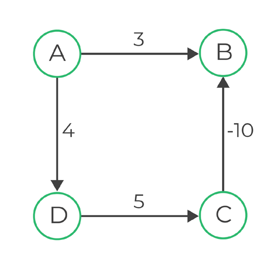
Edges: (A, B), (A, D), (D, C), (C, B)
We can see the values of the distance tabel below
| A | B | C | D |
|---|---|---|---|
| 0 | INF | INF | INF |
Edge (A, B)
0 + 3 < INF => Distance[B] = 3
| A | B | C | D |
|---|---|---|---|
| 0 | 3 | INF | INF |
Edge (A, D)
0 + 4 < INF => Distance[D] = 4
| A | B | C | D |
|---|---|---|---|
| 0 | 3 | INF | 4 |
Edge (D, C)
4 +5 < INF => Distance[C] = 9
| A | B | C | D |
|---|---|---|---|
| 0 | 3 | 9 | 4 |
Edge (C, B)
9-10 < 3 => Distance[B] = -1
| A | B | C | D |
|---|---|---|---|
| 0 | -1 | 9 | 4 |
We can see the values of the distance tabel below
| A | B | C | D |
|---|---|---|---|
| 0 | -1 | 9 | 4 |
Edge (A, B)
0 + 3 < -1 => No, stick with -1
Edge (A, D)
0 + 4 < 4 ? => No, stick with 4
Edge (D, C)
4 +5 < 9 => No, stick with 9
Edge (C, B)
9-10 < -1 => No, stick with -1
No change from previous relaxation, so the answers are final.
                                                int Vertices = 5;

                                                struct Edge {
                                                int source;
                                                int destination;
                                                int weight;
                                                };

                                                class Graph {
                                                public:
                                                using GraphMap = vector<Edge>;
                                                void addEdge(int from, int to, int cost) {
                                                    edges.push_back({ from, to, cost });
                                                }
                                                const GraphMap& getEdges() const { return edges; }
                                                private:
                                                GraphMap edges;
                                                };

                                                void display(const vector<int>& distances) {
                                                std::cout << "Vertex - Distance from Source";
                                                for (int i = 0; i < distances.size(); ++i) {
                                                    cout << i << " - " << distances[i];
                                                }
                                                }

                                                int main() {
                                                Graph graph;
                                                graph.addEdge(0, 1, -1);
                                                graph.addEdge(0, 2, 4);
                                                graph.addEdge(1, 2, 3);
                                                graph.addEdge(1, 3, 2);
                                                graph.addEdge(1, 4, 2);
                                                graph.addEdge(3, 2, 5);
                                                graph.addEdge(3, 1, 1);
                                                graph.addEdge(4, 3, -3);

                                                BellmanFord(graph.getEdges(), 0);
                                                return 0;
                                                }
The main() function starts on line 27.
We have an integer that defines the number of our vertices (Line 1).
We create a graph and add a few edges onto it (Lines 28-36). If we check the implementation of the function (Lines 12-13), we see that the edges are pushed into a vector.
The edge structure contains both the source and the destination (Lines 3-7), therefore we can assume that we are talking about a directed graph.
The algorithm is called on line 38, and the implementation of it can be seen below. The function receives the edges and the source vertex, which in our case will be 0.
                                                void BellmanFord(const Graph::GraphMap& graph, int source) {
                                                    const int MAX_INT = std::numeric_limits<int>::max();
                                                    std::vector<int> distances(Vertices, MAX_INT);
                                                    distances[source] = 0;

                                                    // Iterate through all edges multiple times
                                                    // and update the distances between vertices
                                                    for (int i = 1; i < Vertices - 1; ++i) {
                                                    for (const auto& edge : graph) {
                                                        int src = edge.source;
                                                        int dst = edge.destination;
                                                        int cost = edge.weight;
                                                        if (distances[src] != MAX_INT && distances[src] + cost < distances[dst])
                                                            distances[dst] = distances[src] + cost;
                                                    }
                                                    }
                                                    // final loop for negative cycle detection
                                                    for (const auto& edge : graph) {
                                                    int src = edge.source;
                                                    int dst = edge.destination;
                                                    int cost = edge.weight;
                                                    if (distances[src] != MAX_INT && distances[src] + cost < distances[dst])
                                                        cout << "Negative cycle";
                                                    }

                                                    display(distances);
                                                }
We define MAX_INT as a constant for our highest possible integer (Line 2). This will be used as an initial value for our distances vector, (Line 3), in order to further calculate the smallest distance.
The distances vector has a size of Vertices, so each vertex will have assigned a distance – which is the distance required to reach that vertex from the starting point.
The distance from source to itself is set to 0 (Line 4).
In order to do the relaxation process, we need to iterate through each edge from the graph multiple times (the number of vertices in the graph minus one).
In line 8 we start the iteration process.
For each edge in the graph (Line 8):
Let’s give an example.
Node A is the starting point.
The cost of reaching point B from A is 10. (A-> B = 10)
The cost of reaching point C from B is 2 (B -> C = 2)
The initial cost of reaching point C from A is 30 (A -> C = 30)
If we go from A to B, it will cost 10. If we go from B to C, it will cost 2 more. Therefore, we can reach C by going A -> B -> C, with the total cost of 12. Our current route is direct (A->C) and it costs 30. So let’s update the distance required to reach C, to be 12.
We need to apply the same logic multiple times (the total number of times is the number of vertices), because a change in one step will propagate to the next ones. We will use that updated distance to calculate the distance to other vertices from the graph.
This solution needs to be understood this way:
The condition in line 22 requires that the distance from source point to the node should be different than MAX_INT.
MAX_INT is the default value for our distances vector (except source).
Therefore, the only edges that will pass the condition are the nodes that are directly connected to our source node.
In the next step, we already know the distance to reach the neighbours, and we can use that to get the smallest distance required to reach the 2nd level neighbours (direct connections of direct connections of source node).
By doing this over and over, we will eventually find the smallest distance from our source node to its furthest connection.
The lines 18-24 are the same as the ones above, and they are there to check for negative cycles.
If we already know the value of smallest distances, but we check again and we get different results, it means we have a cycle in the graph that is negative.
Let’s give an example.
{A-> B = 2}, { B-> C = 3}, {C-> A = - 10}.
Going from A to A will take 2+3-10 = -5 distance. Initially we started with 0 distance from A, now we are in the same point with -5.
If we do another loop (A-> B-> C -> A), we will get -5 + 2 + 3 -10 = -10. The distance was again updated, although we haven’t changed anything.
This will go into an infinite loop, because the distance is updated everytime we do another loop.
The travelling salesman problem (TSP) asks the following question: “Given a list of cities and the distances between each pair of cities, what is the shortest possible route that visits each city exactly once and returns to the starting point?”
First step is to choose a node to be our starting/ending point.
Afterwards, we will generate all (n-1)! permutations of cities, where n is the number of cities.
While doing so, we calculate the cost of every permutation and keep track of the minimum cost.
In the end, we return the permutation we have stored, which will be the one with the minimum travelling cost.
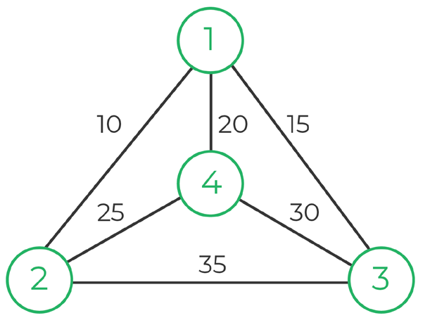
Assuming we have the following graph: We pick 1 as start / end point.
We generate all possible permutations which have 1 as starting and ending point
=> 80 (1-2-4-3-1 / 1-3-4-2-1)
                                                int starting_point = 0;

                                                int TravellingSalesman(vector<vector<int>>& graph, int start) {
                                                vector<int> vertex;
                                                for (int i = 0; i < graph.size(); i++)
                                                    if (i != start)
                                                        vertex.push_back(i);

                                                int minimum_path = std::numeric_limits<int>::max();
                                                do {
                                                    int current_permutation_weight = 0;
                                                    int k = start;
                                                    for (int i = 0; i < vertex.size(); i++) {
                                                        current_permutation_weight += graph[k][vertex[i]];
                                                        k = vertex[i];
                                                    }
                                                    current_permutation_weight += graph[k][start];

                                                    minimum_path = std::min(minimum_path, current_permutation_weight);
                                                } while (std::next_permutation(vertex.begin(), vertex.end()));

                                                return minimum_path;
                                                }

                                                int main() {
                                                vector<vector<int>> graph = {
                                                    { 0, 10, 15, 20 },
                                                    { 10, 0, 35, 25 },
                                                    { 15, 35, 0, 30 },
                                                    { 20, 25, 30, 0 }
                                                };
                                                cout << TravellingSalesman(graph, starting_point);
                                                return 0;
                                                }
The main function, at line 25, will be initially called.
We have a graph which contains the weights from a node x to a node y, where x and y are the rows and columns of the matrix.
For example, we can see that graph[0][4] is 20, which is the weight from node 0 to 4.
We select 0 as starting point in our graph, and we call the TravellingSalesman function.
This function creates a vector and copies all the vertices except our starting point.
This means that, for the nodes {0,1,2,3,4}, the vector will have the values {1,2,3,4}.
We initialize minimum_path with maximum possible value, because we want to overwrite it when we find a path that is less than that.
At the end of the function, we return the minimum path.
Before that, we have the big do – while, which goes on until we have a next permutation for our vector.
This means that we will permute the vector, and its values will change like this:
{1,2,3,4} -> {1,3,2,4} -> {1,4,2,3} …
{2,1,3,4} -> {2,3,1,4} -> {2,3,4,1} …
And so on.
In the do-while, what we’re gonna do is:
At the end, before we go on with the next permutation, we check whether the value of current_permutation_weight is lower than what we have right now, and we overwrite it if so.
Given two sequences, find the length of the longest subsequence that is present in both of them.
A subsequence is a sequence that appears in the same relative order, but not necessarily contiguous.
Let's take an example.
For the string “aeiou”, the following are valid subsequences: “ae”, “aio”, “aiu”, “eu”, “eiu” etc.
Given two strings, one string of length m and one string of length n, we will use a matrix with m+1 rows and n+1 columns, to keep the value of common subsequences.
The first row and first column is initially set to 0.
Assuming we have the first string S1 = “ABCDE”, and the second string S2 = “BAD”.
We can observe the LCS will be of size 2 (“BD”).
Let’s see how we can reach this value.
(S1 = ABCDE)
| String | A | B | C | D | E |
|---|---|---|---|---|---|
| Index | 1 | 2 | 3 | 4 | 5 |
(S2 = BDE)
| String | B | D | E |
|---|---|---|---|
| Index | 1 | 2 | 3 |
We see that I’ve started the index from 1 and not from 0 – that’s because the first row and first column will have their values defaulted to 0.
The algorithm is as follows:
Let’s make this clear with some drawing.
Let’s define a table and set the first rows and columns to 0.
| # | A | B | C | D | E | |
|---|---|---|---|---|---|---|
| # | 0 | 0 | 0 | 0 | 0 | 0 |
| B | 0 | |||||
| D | 0 | |||||
| E | 0 |
Let’s compare S1[1] and S2[1].
A is different than B => do not match, so we take the maximum value between top and left.
S1[1] != S2[1] =>| # | A | B | C | D | E | |
|---|---|---|---|---|---|---|
| # | 0 | 0 | 0 | 0 | 0 | 0 |
| B | 0 | 0 | ||||
| D | 0 | |||||
| E | 0 |
Let’s compare S1[2] and S2[1].
B is the same as B => they match, so we increment 1 to the value of the diagonal.
S1[2] == S2[1] =>
grid[2][1] = 1+ grid[2-1][1-1]
= 1 + 0
= 1
| # | A | B | C | D | E | |
|---|---|---|---|---|---|---|
| # | 0 | 0 | 0 | 0 | 0 | 0 |
| B | 0 | 0 | 1 | |||
| D | 0 | |||||
| E | 0 |
When we compare the remaining entries, we see that they are different characters, so we fill them with max between left and top.
On the left side we have 1, while on the top we have 0, so we fill the remaining entries with 1.
What is that telling us, is that between the strings “ABCDE” and the string “B” we have maximum a subsequence of 1.
Now, we continue for the next digit.
| # | A | B | C | D | E | |
|---|---|---|---|---|---|---|
| # | 0 | 0 | 0 | 0 | 0 | 0 |
| B | 0 | 0 | 1 | 1 | 1 | 1 |
| D | 0 | |||||
| E | 0 |
S1[1] != S2[1] =>
Grid[1][1] = max ( grid[1][0], grid[0][1])
= 0
| # | A | B | C | D | E | |
|---|---|---|---|---|---|---|
| # | 0 | 0 | 0 | 0 | 0 | 0 |
| B | 0 | 0 | 1 | 1 | 1 | 1 |
| D | 0 | 0 | ||||
| E | 0 |
S1[2] != S2[2] =>
Grid[2][2] = max ( grid[2,1], grid[1][2] ) = 1
Why we suddenly have 1 ?
Because although B != D, we already had a subsequence on the top, meaning that:
AB and B have a substring of 1
A and BD have a substring of 0
AB and BD have a substring of 1
| # | A | B | C | D | E | |
|---|---|---|---|---|---|---|
| # | 0 | 0 | 0 | 0 | 0 | 0 |
| B | 0 | 0 | 1 | 1 | 1 | 1 |
| D | 0 | 0 | 1 | |||
| E | 0 |
D and C differ, so we set in the grid the max value between 1 and 1 => 1
| # | A | B | C | D | E | |
|---|---|---|---|---|---|---|
| # | 0 | 0 | 0 | 0 | 0 | 0 |
| B | 0 | 0 | 1 | 1 | 1 | 1 |
| D | 0 | 0 | 1 | 1 | ||
| E | 0 |
D and D are the same character, so we increment the value we had on the diagonal.
| # | A | B | C | D | E | |
|---|---|---|---|---|---|---|
| # | 0 | 0 | 0 | 0 | 0 | 0 |
| B | 0 | 0 | 1 | 1 | 1 | 1 |
| D | 0 | 0 | 1 | 1 | 2 | |
| E | 0 |
D and E differ, so we take the maximum between 2 and 1 => we write 2 in the grid.
That means:
ABCDE and B have a subsequence of 1
ABCD and BD have a subsequence of 2
ABCDE and BD have a subsequence of 2
| # | A | B | C | D | E | |
|---|---|---|---|---|---|---|
| # | 0 | 0 | 0 | 0 | 0 | 0 |
| B | 0 | 0 | 1 | 1 | 1 | 1 |
| D | 0 | 0 | 1 | 1 | 2 | 2 |
| E | 0 |
…And so on
| # | A | B | C | D | E | |
|---|---|---|---|---|---|---|
| # | 0 | 0 | 0 | 0 | 0 | 0 |
| B | 0 | 0 | 1 | 1 | 1 | 1 |
| D | 0 | 0 | 1 | 1 | 2 | 2 |
| E | 0 | 0 | 1 | 1 | 2 | 3 |
We have the following grid, and we start from the lower right.
We see that the last result in the array is 3, meaning that ABCDE and BDE have the longest subsequence of 3.
| # | A | B | C | D | E | |
|---|---|---|---|---|---|---|
| # | 0 | 0 | 0 | 0 | 0 | 0 |
| B | 0 | 0 | 1 | 1 | 1 | 1 |
| D | 0 | 0 | 1 | 1 | 2 | 2 |
| E | 0 | 0 | 1 | 1 | 2 | 3 |
We know the longest subsequence as a number, but now we need to know which letters form the longest subsequence. We find the sequence by finding the values that were incremented from the diagonal, which were in fact the logical step we used when the characters were the same.
We see that the value is different than left and top, meaning that the character was the same, so we got the value by incrementing from diagonal – we mark it and go diagonally.
| # | A | B | C | D | E | |
|---|---|---|---|---|---|---|
| # | 0 | 0 | 0 | 0 | 0 | 0 |
| B | 0 | 0 | 1 | 1 | 1 | 1 |
| D | 0 | 0 | 1 | 1 | 2 | 2 |
| E | 0 | 0 | 1 | 1 | 2 | 3 |
We see that the value is the same as the one from left, so we go left.
| # | A | B | C | D | E | |
|---|---|---|---|---|---|---|
| # | 0 | 0 | 0 | 0 | 0 | 0 |
| B | 0 | 0 | 1 | 1 | 1 | 1 |
| D | 0 | 0 | 1 | 1 | 2 | 2 |
| E | 0 | 0 | 1 | 1 | 2 | 3 |
We see that the value is different than left and top, meaning that the character was the same, so we got the value by incrementing from diagonal – we mark it and go diagonally. We reached the value 0 so we stop there.
| # | A | B | C | D | E | |
|---|---|---|---|---|---|---|
| # | 0 | 0 | 0 | 0 | 0 | 0 |
| B | 0 | 0 | 1 | 1 | 1 | 1 |
| D | 0 | 0 | 1 | 1 | 2 | 2 |
| E | 0 | 0 | 1 | 1 | 2 | 3 |
The values we marked were B, D, and E => BDE is the longest common subsequence.
                                                class Matrix {
                                                    int* arr;
                                                    int width, height;
                                                public:
                                                    Matrix(int x, int y) {
                                                    width = x; height = y;
                                                    arr = new int[x * y] {}; // default to 0
                                                    }
                                                    int& at(int x, int y) const { return arr[x + width * y]; }
                                                };

                                                int lcs(string s1, string s2) {
                                                    const int m = s1.size();
                                                    const int n = s2.size();
                                                    Matrix grid(m + 1, n + 1);

                                                    for (int i = 1; i <= m; i++) {
                                                    for (int j = 1; j <= n; j++) {
                                                        if (s1[i - 1] == s2[j - 1])
                                                            grid.at(i, j) = grid.at(i-1, j-1) + 1;
                                                        else
                                                            grid.at(i, j) = std::max(grid.at(i-1, j), grid.at(i, j-1));
                                                    }
                                                    }

                                                    return grid.at(m, n);
                                                }

                                                int main() {
                                                    string s1 = "ABCDE";
                                                    string s2 = "BDE";

                                                    cout << "LCS = " << lcs(s1, s2);

                                                    return 0;
                                                }
The main() function starts on line 29.
Afterwards, we declare two strings (Lines 30-31) and call the LCS function.
The matrix class (Lines 1-10) is used to store a 2D array. The at() function (Line 9) receives 2 parameters (row and column) and returns the value at that location.
The LCS function starts at line 12.
Then, we get the size of the strings and create the 2d matrix (Lines 13-14).
If we check the line 17-18, we see that we start from index 1. That is because the algorithm behaves this way: the rows and columns with index 0 must have value 0 for our algorithm to work.
That’s the reason why we keep the first row and first column with value 0 – so we can have the algorithm working even when the first character in both strings match (because we will need to access index-1 on both row and column.
At the end, we return the bottom-right location of our matrix, which contains the longest common subsequence.
The rows and the columns are based on the strings we have, so given the first string to be of 3 letters, and 2nd string to be of 5 letters, we will have a matrix of 4x6 (first row and column defaulted to 0, the rest is for each letter in each string).
When we iterate on row, we compare each letter of string 2 to string 1.
When we iterate on column, we compare each letter of string 1 to string 2.
Let’s give an example:
S1 = ABC
S2 = DEF
Row 0, column 0 will have value 0.
Row one will be the longest sequence when we reached the end of S2, but only parsed first letter of S1.
A vs DEF
Column one will be the longest sequence when we reached the end of S1 but only parsed first letter of S2
D vs ABC
Therefore, if the strings have letters in common, we take the maximum between what’s on left and what’s on top until that point.
If strings are ABC, DEF, and we are at location [3][3] (C vs F)
The Floyd-Warshall algorithm is used for finding the shortest path between every pair of vertices in a directed Graph.
The algorithm uses a solution matrix, which is initialized so that the entries correspond to the input graph matrix.
Assuming A is the source vertex and B is the destination, we need to find the shortest distance from A to B.
The shortest path could be by going directly from A to B. However, this may not be always the case, and a more efficient solution would be to go through one or multiple other vertices first, such as: A->C->B, or A->D->C->B
This algorithm moves the source vertex as the middle vertex -> The shortest path that reaches B by going through A.
Let’s create a matrix that contains the distances that we have.
In the matrix we will have the following digits:
| # | A | B | C | D |
|---|---|---|---|---|
| A | ||||
| B | ||||
| C | ||||
| D |
Let’s fill the matrix now:
Self-loop -> 0’s
| # | A | B | C | D |
|---|---|---|---|---|
| A | 0 | |||
| B | 0 | |||
| C | 0 | |||
| D | 0 |
No edge - infinity
| # | A | B | C | D |
|---|---|---|---|---|
| A | 0 | INF | INF | |
| B | 0 | INF | ||
| C | INF | 0 | ||
| D | INF | INF | 0 |
Edge between vertices – write the cost
| # | A | B | C | D |
|---|---|---|---|---|
| A | 0 | 5 | INF | INF |
| B | 7 | 0 | 2 | INF |
| C | 6 | INF | 0 | 1 |
| D | 8 | INF | INF | 0 |
So now we have this solution matrix that represents our graph, and we will use it to calculate the shortest path from one source to all the other vertices.
| # | A | B | C | D |
|---|---|---|---|---|
| A | 0 | 5 | INF | INF |
| B | 7 | 0 | 2 | INF |
| C | 6 | INF | 0 | 1 |
| D | 8 | INF | INF | 0 |
Let’s assume the source vertex is A – we copy the values we had on that row and column, and also the 0’s we had for the self loops.
Now let’s calculate the paths, starting with the first unset position (B, C)
| # | A | B | C | D |
|---|---|---|---|---|
| A | 0 | 5 | INF | INF |
| B | 7 | 0 | ||
| C | 6 | 0 | ||
| D | 8 | 0 |
We see in the solution matrix that the value that we have is 2.
The shortest path is the minimum value between the initial one (2) and the sum of vertices where the source is added in-between.
Let’s see what that means.
We need to calculate [B,C]
We know [B, C] is 2.
The source vertex is A.
Let’s replace each edge with A, and calculate the sum of these values.
Replacing [B, C] =
[A, C] in the solution table = infinity
[B, A] in the solution table = 7
The shortest path for [B, C]:
Min([B, C], [B, A] + [A, C]) = Min( 2, (infinity + 7)
=> It’s clear that 2 is the minimum value.
| # | A | B | C | D |
|---|---|---|---|---|
| A | 0 | 5 | INF | INF |
| B | 7 | 0 | 2 | |
| C | 6 | 0 | ||
| D | 8 | 0 |
The shortest path for [B,D]:
Min (INF, [B, A] + [A, D] ) = Min( INF, 7 + INF)
=> INF
| # | A | B | C | D |
|---|---|---|---|---|
| A | 0 | 5 | INF | INF |
| B | 7 | 0 | 2 | INF |
| C | 6 | 0 | ||
| D | 8 | 0 |
The shortest path for [C, B]:
Min (INF, [C, A] + [A, B]) = Min( INF, 6 + 5)
=> 11
| # | A | B | C | D |
|---|---|---|---|---|
| A | 0 | 5 | INF | INF |
| B | 7 | 0 | 2 | INF |
| C | 6 | 11 | 0 | |
| D | 8 | 0 |
The shortest path for [C, D]:
Min (1, [C,A] + [A, D]) = Min(1, 6 + INF)
=> 1
| # | A | B | C | D |
|---|---|---|---|---|
| A | 0 | 5 | INF | INF |
| B | 7 | 0 | 2 | INF |
| C | 6 | 11 | 0 | 1 |
| D | 8 | 0 |
The shortest path for [D, B]:
Min (INF, [D, A] + [A, B]) = Min(INF, 8 + 5)
=> 13
| # | A | B | C | D |
|---|---|---|---|---|
| A | 0 | 5 | INF | INF |
| B | 7 | 0 | 2 | INF |
| C | 6 | 11 | 0 | 1 |
| D | 8 | 13 | 0 |
The shortest path for [D, C]:
Min (INF, [D, A] + [A, C]) = Min(INF, 8 + INF)
=> INF
| # | A | B | C | D |
|---|---|---|---|---|
| A | 0 | 5 | INF | INF |
| B | 7 | 0 | 2 | INF |
| C | 6 | 11 | 0 | 1 |
| D | 8 | 13 | INF | 0 |
If we continue and select the next node as starting node, we will keep updating the table. In the end, the table will look like this:
| # | A | B | C | D |
|---|---|---|---|---|
| A | 0 | 5 | 7 | 8 |
| B | 7 | 0 | 2 | 3 |
| C | 6 | 11 | 0 | 1 |
| D | 8 | 13 | 15 | 0 |
The values that were infinity are now small, finite numbers.
We understand why the first row/column were infinite, since we never calculated them, but what about BD, and DC?
BD = min(INF, BA + AD)
> AD was infinite because it was never calculated
> BD is also infinite at first iteration
DC = min(INF, DA + AC)
> AC was infinite because it was never calculated
> DC is also infinite at first iteration
                                                    int INF = 99999;

                                                    void display(vector<vector<int>> & graph) {
                                                    for (const auto& items : graph) {
                                                        for (const auto& item : items) {
                                                            if (item == INF)
                                                                cout << "INF ";
                                                            else
                                                                cout << item << " ";
                                                        }
                                                    }
                                                    }

                                                    void floydWarshall(vector<vector<int>> & graph) {
                                                    const int len = graph.size();

                                                    for (int k = 0; k < len; k++) {
                                                        for (int i = 0; i < len; i++) {
                                                            for (int j = 0; j < len; j++) {
                                                                graph[i][j] = std::min(graph[i][j], graph[i][k] + graph[k][j]);
                                                            }
                                                        }
                                                    }
                                                    display(graph);
                                                    }

                                                    int main() {
                                                        vector<vector<int>> graph = {
                                                        { 0, 5, INF, INF },
                                                        { 7, 0, 2, INF },
                                                        { 6, INF, 0, 1 },
                                                        { 8, INF, INF, 0 }
                                                        };

                                                    floydWarshall(graph);
                                                    return 0;
                                                    }
The main() function starts on line 27.
Afterwards, we create a graph, by using a vector of vectors – in other words, a two-dimensional matrix, which contains the distances from one node to another. (eg. Item on row = 3, column = 4, is the edge cost from node 3 to node 4. The value 0 is used for the distance from node to self (row equal to column). In case there’s no edge between two given vertices, the INF value is used. This value is defined on line 1.
Why did we not use something such as the max integer value? We could have used that, but I wanted to make the algorithm as simple as possible.
Explanation:
In line 20, we will have a sum of values, and adding any positive value with the highest possible value that can be written with those bits will cause an integer overflow, so we’ll go on the negative side.
This would have required for the algorithm to become more complex, checking for such overflows and so on.
In line 35, we call the floydWarshall() function, which will create the solution for us.
The display() function from lines 3-12 receives the graph as parameter and iterates through it, displaying its values.
Ok, let’s go to the function we’re interested in – floydWarshall (Line 14).
Line 17 will simply do the same logic over and over again – for X times, where X is the number of vertices we have.
In line 18 and 19, we iterate through our 2d matrix – and update the edge cost, based on the information we have at that point.
Let’s read the code from line 20:
The value of graph[i][j] (the cost required to get from node i to node j) is, either the current value, if that’s the smallest one, either the sum of the costs by reaching that point through an intermediary node.
And that’s why we have the line 17 -> each node will be, at some point, the intermediary node for each traversal.
So, what we’re actually saying, is that:
Assuming k=1, i=2, j=3 =>
Vertex: Node containing data
Edge: The line that connects two vertices
Cycle: Cycles occur when nodes are connected in a way that they forms a closed structure.
Cycle: Cycles occur when nodes are connected in a way that they forms a closed structure.
Self loop: An edge that connects a vertex to itself (source = destination).
Divide et impera (Divide and conquer): Break the problem into sub-problems and solve them each recursively.
Negative weight edge refer to edges with a negative cost.